|
Size: 9116
Comment:
|
Size: 15729
Comment:
|
| Deletions are marked like this. | Additions are marked like this. |
| Line 5: | Line 5: |
*[[attachment:GSEA_paper2005.pdf]] |
|
| Line 13: | Line 11: |
| *adapted from http://www.broadinstitute.org/cancer/software/genepattern/modules/docs/GSEA/14 |
|
| Line 15: | Line 15: |
| GSEA has been first developped to interpret results from microarray experiments. One common approach to analyzing these data is to identify a limited number of the most interesting genes by picking a significance cutoff that will trim the list of interesting genes down to a handful of genes for further research. Gene Set Enrichment Analysis (GSEA) takes an alternative approach : it focuses on cumulative changes in expression of multiple genes as a group (belonging to a same gene-set/pahtway), which shifts the focus from individual genes to groups of genes. By looking at several genes at once, GSEA can identify pathways whose several genes each change a small amount, but in a coordinated way. | *GSEA has been first developped to interpret results from microarray experiments. One common approach to analyzing these data is to identify a limited number of the most interesting genes by picking a significance cutoff that will trim the list of interesting genes down to a handful of genes for further research. Gene Set Enrichment Analysis (GSEA) takes an alternative approach : it focuses on cumulative changes in expression of multiple genes as a group (belonging to a same gene-set/pahtway), which shifts the focus from individual genes to groups of genes. By looking at several genes at once, GSEA can identify pathways whose several genes each change a small amount, but in a coordinated way. *adapted from http://www.broadinstitute.org/cancer/software/genepattern/modules/docs/GSEA/14 |
| Line 21: | Line 23: |
| *adapted from http://www.broadinstitute.org/cancer/software/genepattern/modules/docs/GSEA/14 |
|
| Line 22: | Line 27: |
| {{attachment:content_gseapic1.png}} | |
| Line 42: | Line 48: |
| * which values to consider for interpretating results: | *[[attachment:GSEA_paper2005.pdf]]: equations and definition for statistics calculated by GSEA are described at the end of the paper as supplemental information. * GSEA plot: {{attachment:GSEAplot.gif}} * which values to consider for interpreting results: |
| Line 58: | Line 71: |
| * relationships between ES, pvalue , NES and FDR: * pvalue is calculated from ES * FDR is calculated from NES * the higher the ES or NES and the lowest the FDR or pvalue * NES above 1.4 will usually give significant results |
|
| Line 83: | Line 101: |
| === Required fields === * Expression dataset: contains the normalized data in a .GCT format * Gene sets database: contains information about all the pathways that are going to be tested. We use the Baderlab collection for this exercise but Msig databases are also available here. * Number of permutations: 100 for a short run time for practical reason during this lab: use 1000 or 2000 in real life! It is used to calculate the significance of the enrichment, i.e the calculation of the pvalue and FDR. * Phenotype labels: tells GSEA which 2 groups of samples we would like to compare (treated at 12hours and non treated at 12 hours in this exercise) * Collapse dataset to gene symbols: set to false in this exercise because we already substituted probe ID by Gene Symbol in the GCT file while preparing files for this lab. If you have probe id as your first column and not the gene names, set Collapse dataset to gene symbols to true and choose the corresponding Chip platform. * Permutation type: set to gene-set as we don’t have enough samples to run successfully phenotype permutation (try phenotype permutation if you have more than 20 samples per group of comparison) * Chip platform(s): stays empty if Collapse dataset to gene symbol if set to false. Otherwise, you need to retrieve your chip model using this link. === Basic fields === * Analysis name: self explanatory *Enrichment statistic : weighted is the default and is equivalent to a weight of 1. the genes that are top ranked will contribute with a greater amplitude to the enrichment score. It is a good idea to change the weight to p2 for noisier data to increase confidence about the results. It is not recommended to use a weight of 0. *Metric for ranking genes: ‘tTest’ is recommended. A fold change metric can be tried for noisy data where no significant results could be obtained using the t-test (Ratio_of_Classes for linear data format and Diff_of_Classes for log scale data format). *Gene list sorting mode: ‘real’ means that genes associated with with positive t values will be ranked at the top of the gene list and genes with negative t values at the very bottom of the list. It indicates that we are looking for enrichment in gene-sets separately for genes that are up-regulated (positive phenotype) and genes that are down-regulated (negative phenotype). If you are interested to look for enrichment in genes differentially expressed regardless of up- or down-regulation, set the sorting mode to’ abs’. *Gene list ordering mode: set to descending. It will rank the list from positive t values at the top of the list to negative t values at the bottom. Ascending will do the reverse. *Max size: exclude larger sets: set to 500. Larger gene-sets may be too generic to be informative. It could correspond to higher level terms such as ‘cell’, ‘plasma membrane’ or ‘biological process’ *Min size: exclude smaller sets: set to 15. GSEA statistics will not be reliable for gene-set containing a small number of genes. *Save results in this folder: self explanatory. === Advanced fieds === *Collapsing mode for probe sets => 1 gene: Max_probe . On a chip (Illumina or Affymetrix) multiple probes are designed to target a same gene. However, no duplicated genes are allowed in the data when gene-set enrichment is performed. Max_probe will select the probe with the highest rank. *Normalization mode: meandiv. It used to calculate the normalized enrichment score (NES) from the enrichment score (ES). (http://www.broadinstitute.org/gsea/doc/GSEAUserGuideTEXT.htm#_Normalized_Enrichment_Score) *Randomization mode: no_balance. Method used to normalize the enrichment scores across analyzed gene sets. It us not used when ‘Permutation type’ is set to ‘gene-set’. *omit features with no symbol match: Used only when collapse dataset is set to true. By default (true), the new dataset excludes probes/genes that have no gene symbols. *make detailed gene set report: Create detailed gene set report (heat map, mountain plot, etc.) for each enriched gene set. *median for class metrics: Specifies whether to use the median of each class, instead of the mean, in the metric for ranking genes. Default: false *number of markers Number of features (gene or probes) to include in the butterfly plot in the Gene Markers section of the gene set enrichment report. Default: 100 *plot graphs for the top sets of each phenotype Generates summary plots and detailed analysis results for the top x genes in each phenotype, where x is 20 by default. The top genes are those with the largest normalized enrichment scores. Default: 20 *random seed: Seed used to generate a random number for phenotype and gene_set permutations. Timestamp is the default. Using a specific integer valued seed generates consistent results, which is useful when testing software. *save random ranked lists: Specifies whether to save the random ranked lists of genes created by phenotype permutations. *output file name Name of the output file. The name cannot include spaces. == Link to EnrichmentMap tutorials: how to create using GSEA results == TODO == what is single sample GSEA == |
|
| Line 85: | Line 140: |
| == what is single sample GSEA == TODO |
== References == * Subramanian A, Tamayo P, Mootha VK, Mukherjee S, Ebert BL, Gillette MA, Paulovich A, Pomeroy SL, Golub TR, Lander ES, Mesirov JP. Gene set enrichment analysis: A knowledge-based approach for interpreting genome-wide expression profiles. PNAS. 2005;102(43);15545-15550. *[[attachment:GSEA_paper2005.pdf]]: equations and definition for statistics calculated by GSEA are described at the end of the paper as supplemental information. * GSEA documentation: http://www.broadinstitute.org/gsea/doc/GSEAUserGuideFrame.html * A more condensed document is available at http://www.broadinstitute.org/cancer/software/genepattern/modules/docs/GSEA/14 |
GSEA Gene Set Enrichment Analysis (www.broadinstitute.org/gsea )
Contents
-
GSEA Gene Set Enrichment Analysis (www.broadinstitute.org/gsea )
- Summary
- Introduction
- Method
- GSEA enrichment scores and statistics
- GSEA formats (.GCT, .CLS, .RNK, .GMT) :
- Tips on how to install GSEA locally and launch it from the command line:
- GSEA parameters
- Link to EnrichmentMap tutorials: how to create using GSEA results
- what is single sample GSEA
- References
- Answers to questions
- Troubleshooting
Summary
- Gene Set Enrichment Analysis (GSEA) is a method for calculating gene-set enrichment.GSEA first ranks all genes in a data set, then calculates an enrichment score for each gene-set (pathway), which reflects how often members (genes) included in that gene-set (pathway) occur at the top or bottom of the ranked data set (for example, in expression data, in either the most highly expressed genes (top) or the most underexpressed genes(bottom).
adapted from http://www.broadinstitute.org/cancer/software/genepattern/modules/docs/GSEA/14
Introduction
- GSEA has been first developped to interpret results from microarray experiments. One common approach to analyzing these data is to identify a limited number of the most interesting genes by picking a significance cutoff that will trim the list of interesting genes down to a handful of genes for further research. Gene Set Enrichment Analysis (GSEA) takes an alternative approach : it focuses on cumulative changes in expression of multiple genes as a group (belonging to a same gene-set/pahtway), which shifts the focus from individual genes to groups of genes. By looking at several genes at once, GSEA can identify pathways whose several genes each change a small amount, but in a coordinated way.
adapted from http://www.broadinstitute.org/cancer/software/genepattern/modules/docs/GSEA/14
Method
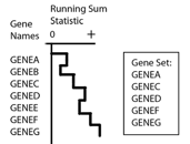
GSEA first ranks the genes based on a measure of each gene's differential expression with respect to the two phenotypes (for example, tumor versus normal using a t-test) or correlation with a continuous phenotype. Then the entire ranked list is used to assess how the genes of each gene set are distributed across the ranked list. To do this, GSEA walks down the ranked list of genes, increasing a running-sum statistic when a gene belongs to the set and decreasing it when the gene does not.
A simplified example is shown in the following figure.
The enrichment score (ES) is the maximum deviation from zero encountered during that walk. The ES reflects the degree to which the genes in a gene set are overrepresented at the top or bottom of the entire ranked list of genes. A set that is not enriched will have its genes spread more or less uniformly through the ranked list. An enriched set, on the other hand, will have a larger portion of its genes at one or the other end of the ranked list. The extent of enrichment is captured mathematically as the ES statistic.
Next, GSEA estimates the statistical significance of the ES by a permutation test. To do this, GSEA creates a version of the data set with phenotype labels randomly scrambled, produces the corresponding ranked list, and recomputes the ES of the gene set for this permuted data set. GSEA repeats this many times (1000 is the default) and produces an empirical null distribution of ES scores. Alternatively, permutations may be generated by creating “random” gene sets (genes randomly selected from those in the expression dataset) of equal size to the gene set under analysis.
The nominal p-value estimates the statistical significance of a single gene set's enrichment score, based on the permutation-generated null distribution. The nominal p-value is the probability under the null distribution of obtaining an ES value that is as strong or stronger than that observed for your experiment under the permutation-generated null distribution.
Typically, GSEA is run with a large number of gene sets. For example, the MSigDB collection and subcollections each contain hundreds to thousands of gene sets. This has implications when comparing enrichment results for the many sets:
The ES must be adjusted to account for differences in the gene set sizes and in correlations between gene sets and the expression data set. The resulting normalized enrichment scores (NES) allow you to compare the analysis results across gene sets.
The nominal p-values need to be corrected to adjust for multiple hypothesis testing. For a large number of sets (rule of thumb: more than 30), we recommend paying attention to the False Discovery Rate (FDR) q-values: consider a set significantly enriched if its NES has an FDR q-value below 0.25.
GSEA enrichment scores and statistics
GSEA_paper2005.pdf: equations and definition for statistics calculated by GSEA are described at the end of the paper as supplemental information.
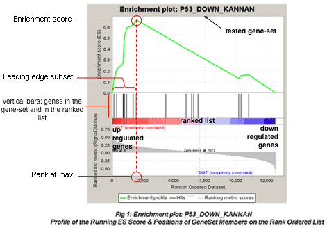
- GSEA plot:

- which values to consider for interpreting results:
number of gene-set tested |
1 gene-set |
few gene-sets (3-10) |
a lot of gene-sets >3000 |
ES |
|
not recommended |
not recommended |
NES |
not informative |
|
|
nom p-value |
|
better to use FDR |
better to use FDR |
FDR |
not informative |
|
|
(*) FDR values are going to be pessimistic when using the BaderLab geneset files due to the high number of tested gene-sets and therefore the high p-value adjustment needed.
- ES (enrichment score): reflects the degree to which a gene-set is overrepresented at the top or bottom of a ranked list of genes.
- NES (normalized enrichment score): NES corrects for differences in ES between gene-sets due to differences in gene-set sizes. It enables to compare the scores of the different tested gene-sets with each other.
- NES = actual ES / mean of all ESs obtained from all random permutations for the single gene-set that is being tested
- nom p-value: The nominal p value estimates the statistical significance of the enrichment score for a single gene set. The p-value is calculated from the null distribution.
- Using gene-set permutation, the null distribution is created by generating, for each permutation, a random gene set the same size as your specified gene set by selecting that number of genes from all of the genes in your expression data set (or pre-ranked list), and then calculating the enrichment score for that randomly selected gene set. The distribution of those enrichment scores across all of the permutations constitutes the null distribution.
- FDR: corrects for multiple hypothesis testing and enable a more correct comparison of the different tested gene-sets with each other.
note: for a given gene-set S and observed NES, called NES*, FDR is [% of all NES (including permutations) >= NES*] / [% of all observed NES (=NES for all tested gene-sets) >= NES*]
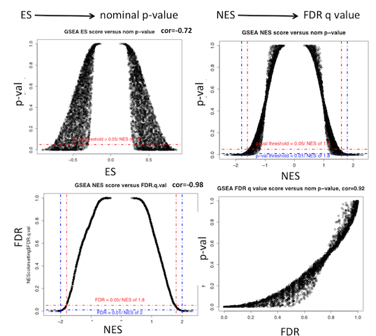
- relationships between ES, pvalue , NES and FDR:
- pvalue is calculated from ES
- FDR is calculated from NES
- the higher the ES or NES and the lowest the FDR or pvalue
- NES above 1.4 will usually give significant results

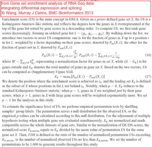
Explanation of GSEA ES score and values from Wang and Murray (BMC Bioinformatics 2013):
GSEA formats (.GCT, .CLS, .RNK, .GMT) :
http://www.broadinstitute.org/cancer/software/gsea/wiki/index.php/Data_formats
http://www.broadinstitute.org/cancer/software/genepattern/modules/docs/GSEA/14
Tips on how to install GSEA locally and launch it from the command line:
- Download and Save the gsea2-2.0.14.jar file in your folder Documents
- open your console/terminal window
- Type the command for MAC:
- "java -Xmx2G -jar ~/Documents/gsea2-2.0.14.jar"
- Type the command for Windows:
- "cd Documents"
- "java -Xmx2G –jar gsea2-2.0.14.jar"
GSEA parameters
Required fields
- Expression dataset: contains the normalized data in a .GCT format
- Gene sets database: contains information about all the pathways that are going to be tested. We use the Baderlab collection for this exercise but Msig databases are also available here.
- Number of permutations: 100 for a short run time for practical reason during this lab: use 1000 or 2000 in real life! It is used to calculate the significance of the enrichment, i.e the calculation of the pvalue and FDR.
- Phenotype labels: tells GSEA which 2 groups of samples we would like to compare (treated at 12hours and non treated at 12 hours in this exercise)
- Collapse dataset to gene symbols: set to false in this exercise because we already substituted probe ID by Gene Symbol in the GCT file while preparing files for this lab. If you have probe id as your first column and not the gene names, set Collapse dataset to gene symbols to true and choose the corresponding Chip platform.
- Permutation type: set to gene-set as we don’t have enough samples to run successfully phenotype permutation (try phenotype permutation if you have more than 20 samples per group of comparison)
- Chip platform(s): stays empty if Collapse dataset to gene symbol if set to false. Otherwise, you need to retrieve your chip model using this link.
Basic fields
- Analysis name: self explanatory
- Enrichment statistic : weighted is the default and is equivalent to a weight of 1. the genes that are top ranked will contribute with a greater amplitude to the enrichment score. It is a good idea to change the weight to p2 for noisier data to increase confidence about the results. It is not recommended to use a weight of 0.
- Metric for ranking genes: ‘tTest’ is recommended. A fold change metric can be tried for noisy data where no significant results could be obtained using the t-test (Ratio_of_Classes for linear data format and Diff_of_Classes for log scale data format).
- Gene list sorting mode: ‘real’ means that genes associated with with positive t values will be ranked at the top of the gene list and genes with negative t values at the very bottom of the list. It indicates that we are looking for enrichment in gene-sets separately for genes that are up-regulated (positive phenotype) and genes that are down-regulated (negative phenotype). If you are interested to look for enrichment in genes differentially expressed regardless of up- or down-regulation, set the sorting mode to’ abs’.
- Gene list ordering mode: set to descending. It will rank the list from positive t values at the top of the list to negative t values at the bottom. Ascending will do the reverse.
- Max size: exclude larger sets: set to 500. Larger gene-sets may be too generic to be informative. It could correspond to higher level terms such as ‘cell’, ‘plasma membrane’ or ‘biological process’
- Min size: exclude smaller sets: set to 15. GSEA statistics will not be reliable for gene-set containing a small number of genes.
- Save results in this folder: self explanatory.
Advanced fieds
Collapsing mode for probe sets => 1 gene: Max_probe . On a chip (Illumina or Affymetrix) multiple probes are designed to target a same gene. However, no duplicated genes are allowed in the data when gene-set enrichment is performed. Max_probe will select the probe with the highest rank.
Normalization mode: meandiv. It used to calculate the normalized enrichment score (NES) from the enrichment score (ES). (http://www.broadinstitute.org/gsea/doc/GSEAUserGuideTEXT.htm#_Normalized_Enrichment_Score)
- Randomization mode: no_balance. Method used to normalize the enrichment scores across analyzed gene sets. It us not used when ‘Permutation type’ is set to ‘gene-set’.
- omit features with no symbol match: Used only when collapse dataset is set to true. By default (true), the new dataset excludes probes/genes that have no gene symbols.
- make detailed gene set report: Create detailed gene set report (heat map, mountain plot, etc.) for each enriched gene set.
- median for class metrics: Specifies whether to use the median of each class, instead of the mean, in the metric for ranking genes. Default: false
- number of markers Number of features (gene or probes) to include in the butterfly plot in the Gene Markers section of the gene set enrichment report. Default: 100
- plot graphs for the top sets of each phenotype Generates summary plots and detailed analysis results for the top x genes in each phenotype, where x is 20 by default. The top genes are those with the largest normalized enrichment scores. Default: 20
- random seed: Seed used to generate a random number for phenotype and gene_set permutations. Timestamp is the default. Using a specific integer valued seed generates consistent results, which is useful when testing software.
- save random ranked lists: Specifies whether to save the random ranked lists of genes created by phenotype permutations.
- output file name Name of the output file. The name cannot include spaces.
Link to EnrichmentMap tutorials: how to create using GSEA results
TODO
what is single sample GSEA
TODO
References
- Subramanian A, Tamayo P, Mootha VK, Mukherjee S, Ebert BL, Gillette MA, Paulovich A, Pomeroy SL, Golub TR, Lander ES, Mesirov JP. Gene set enrichment analysis: A knowledge-based approach for interpreting genome-wide expression profiles. PNAS. 2005;102(43);15545-15550.
GSEA_paper2005.pdf: equations and definition for statistics calculated by GSEA are described at the end of the paper as supplemental information.
GSEA documentation: http://www.broadinstitute.org/gsea/doc/GSEAUserGuideFrame.html
A more condensed document is available at http://www.broadinstitute.org/cancer/software/genepattern/modules/docs/GSEA/14
Answers to questions
- Question: how can we compare the NES (same gene-sets) between different datasets:
1) single sample GSEA case: e.g single sample GSEA was used on several patients and then a matrix of NES is created with the gene-sets as rows and patients as column and you want to find out gene-sets that are comparable between patients. A t-test with 1 group could be used to identify the gene-sets with comparable NES throughout samples --> t = mean/ standard error. The gene-sets will get a pvalue close to 0 only for gene-sets with comparable NES across patients (standard error is going to be small)
- 2) GSEA has been run using GSEA preranked option, you created a map using the 2 datasets and you see that the map is similar (e.g JAK2 responders versus partial responders) (high correlation throughout the gene-sets for the 2 datasets). You can do a K_S (Kolmogorov–Smirnov) test or a Wilcoxon rank sum test on the NES from the 2 datasets to see if "the 2 maps" are different or not.
Troubleshooting
- out of memory:
- running GSEA using the comprehensive Baderlab gene-set is using 1.8 GB of memory:
- Check that you have at least 2GB of free memory on your machine
- Check that you haved allocated enough memory to GSEA when launching GSEA
- using the javaGSEA Desktop Application: Launch with 2GB (for 64-bit Java only)
using the javaGSEA jar file: allocate 2GB of memory using this command: "java -Xmx2G –jar gsea2-2.0.14.jar"
- running GSEA using the comprehensive Baderlab gene-set is using 1.8 GB of memory:
- java version:
- GSEA works with java 6 , java 7 and java 8. However, for java 7 and 8, launching GSEA using the javaGSEA Desktop may not work because on some security settings on your computer, in this case try to launch GSEA using the command line.


